Reccurent Neural Network (LSTM) in Tensorflow
This unit is using the MNIST database of handwritten digits (http://yann.lecun.com/exdb/mnist/)
Tensorflow code courtesy of MorvanZhou. We have added some more annotations and graphic illustrations of the mnist dataset. We have also added result analysis and ideas for course projects.
MorvanZhou
can be downloaded from this link:
https://github.com/aymericdamien/TensorFlow-Examples/blob/master/examples/3_NeuralNetworks/recurrent_network.py
MorvanZhou code is a very good one for RNN beginners. Feel free to check it out (by his recommendation).
View more python learning tutorial on his Youtube and Youku channel:
- Youtube video tutorial: https://www.youtube.com/channel/UCdyjiB5H8Pu7aDTNVXTTpcg
- Youku channel: http://i.youku.com/pythontutorial
Other links to good tutorials on RNN (and LSTM networks):
# These are css/html styles for good looking ipython notebooks
from IPython.core.display import HTML
css = open('style-notebook.css').read()
HTML('<style>{}</style>'.format(css))
import tensorflow as tf
from tensorflow.examples.tutorials.mnist import input_data

# set random seed for comparing the two result calculations
tf.set_random_seed(1)
Loading the mnist data
mnist = input_data.read_data_sets('MNIST_data', one_hot=True)
The mnist object is a special Tensorflow object which contains 55000 digit images for training and 10000 images for validation
- mnist.train.images
- mnist.test.images
type(mnist)
mnist.train.images.shape
mnist.test.images.shape
mnist.train.labels[8].argmax() # a simple way to get the label from a one-hot vector
Lets draw a few of these images, in order to get acquainted with the data
import matplotlib.pyplot as plt
plt.rcParams['figure.figsize'] = (8,7)
%matplotlib inline

def draw_digit(x):
    img = x.reshape(28,28)
    plt.imshow(img, cmap='gray', interpolation='none')
digit = mnist.train.images[0]
draw_digit(digit)

Sometimes we want to draw a larger group of digits
def draw_digits(digits, labels, n_rows=3):
    n = len(digits)
    n_cols = int(n / n_rows)
    for i in range(0, n):
        plt.subplot(n_rows, n_cols, i+1)
        img = digits[i].reshape(28,28)
        label = labels[i].argmax()
        plt.imshow(img, cmap='gray', interpolation='none')
        plt.title(label, fontsize=12)
        plt.tick_params(axis='both', which='major', labelsize=6)
        plt.subplots_adjust(hspace=0.0, wspace=0.5)
Let's look at 24 examples of digits and their labels. We simply choose to see the digits located at locations 500 to 523 in our dataset:
plt.rcParams['figure.figsize'] = (8,7)
digits = mnist.train.images[500:524]
labels = mnist.train.labels[500:524]
draw_digits(digits, labels, n_rows=4)

Hyperparameters
lr = 0.001                   # learning rate
training_iters = 100000      # Number of training
batch_size = 128             # Batch size
n_inputs = 28                # MNIST data input (img shape: 28*28)
n_steps = 28                 # Time steps for recurrent cell
n_hidden_units = 128         # Number of neurons in hidden layer
n_classes = 10               # MNIST classes (0-9 digits): 0, 1, 2, 3, ..., 9
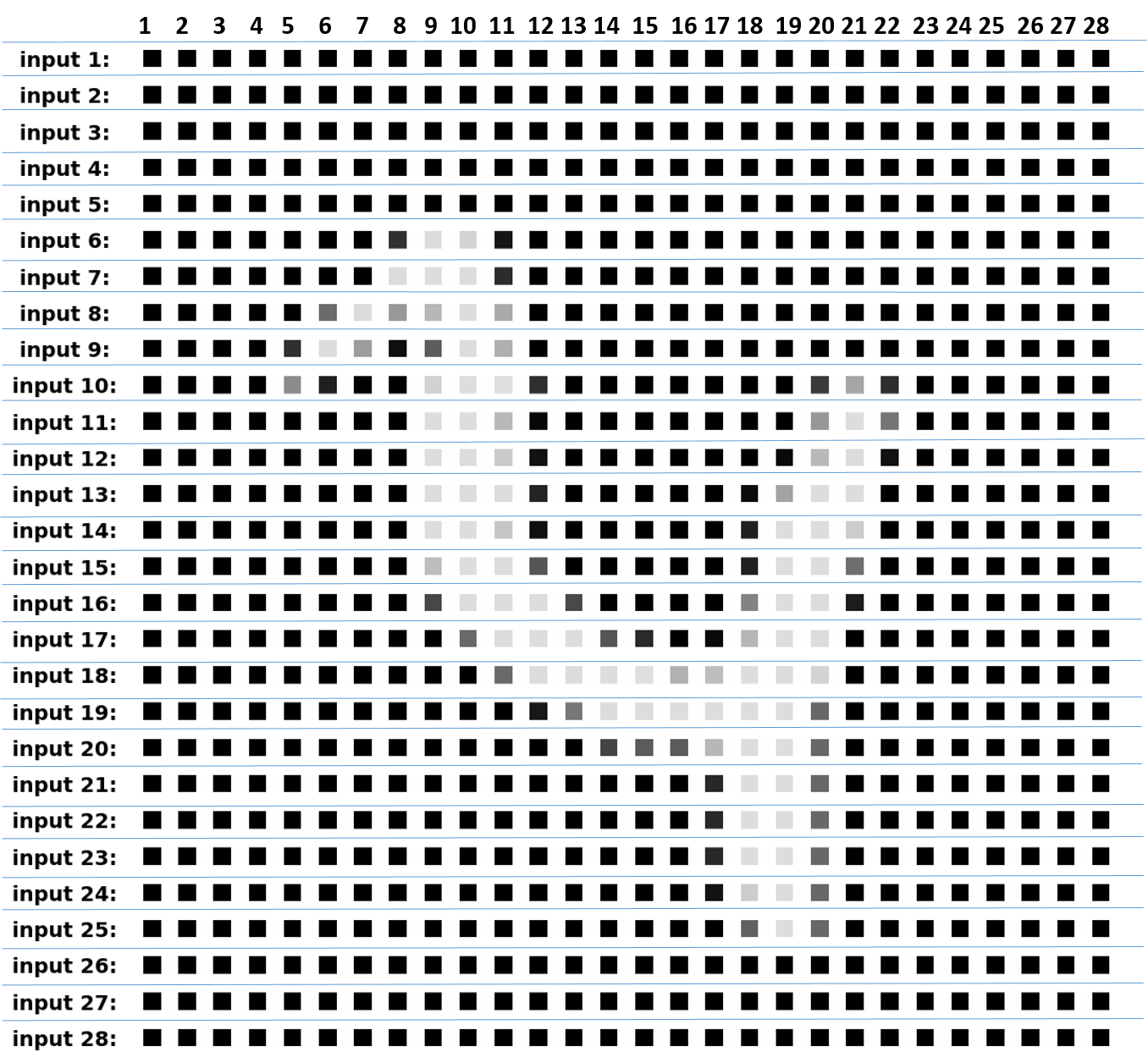
Each MNIST digit image has a 28x28 pixels shape. It will be fed to our LSTM cell in 28 time steps. At each step, the LSTM cell will process one row (1x28 pixels), as can be seen from the following illustration. Each row is a vector of 28 gray pixels. Every gray square represents one gray pixel with color intensity between 0.0 to 1.0.
Tensorflow graph definition
# tf Graph inputs
x = tf.placeholder(tf.float32, [None, n_steps, n_inputs])
y = tf.placeholder(tf.float32, [None, n_classes])

# Define weights matrices
weights = {
    # matrix from inputs (28) to hidden layer (128). shape is: (28, 128)
    'in': tf.Variable(tf.random_normal([n_inputs, n_hidden_units])),
    # matrix from hidden layer to output layer, shape is: (128, 10)
    'out': tf.Variable(tf.random_normal([n_hidden_units, n_classes]))
}

# Define bias vectors
biases = {
    # bias for the input to hidden layer (128, )
    'in': tf.Variable(tf.constant(0.1, shape=[n_hidden_units, ])),
    # bias from the hidden to putput layer (10, )
    'out': tf.Variable(tf.constant(0.1, shape=[n_classes, ]))
}
Defining the RNN (Recurrent Neural Network)
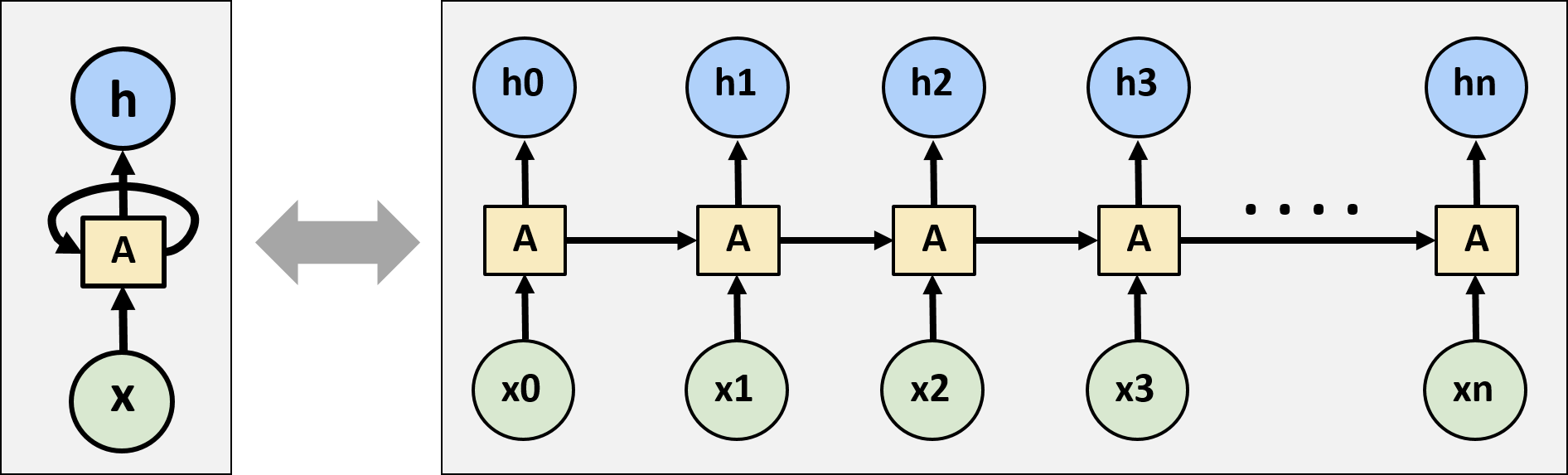
def RNN(X, weights, biases):
    # hidden layer for input to lstm cell

    # transpose the inputs shape from 3D [batch, steps, inputs]
    # to 2D: [(128 batch * 28 steps), 28 inputs)
    # new shape: [128*28, 28]
    X = tf.reshape(X, [-1, n_inputs])

    # flow from input layer to hidden layer
    # X_in = (128 batch * 28 steps, 128 hidden)
    X_in = tf.matmul(X, weights['in']) + biases['in']
    # X_in ==> (128 batch, 28 steps, 128 hidden)
    X_in = tf.reshape(X_in, [-1, n_steps, n_hidden_units])

    # basic LSTM Cell
    lstm_cell = tf.nn.rnn_cell.BasicLSTMCell(n_hidden_units, forget_bias=1.0, state_is_tuple=True)
    # lstm cell is divided into two parts (c_state, h_state)
    init_state = lstm_cell.zero_state(batch_size, dtype=tf.float32)

    # You have 2 options for following step.
    # 1: tf.nn.rnn(cell, inputs);
    # 2: tf.nn.dynamic_rnn(cell, inputs).
    # In option 1, you have to modify the shape of X_in, go and check out this:
    # https://github.com/aymericdamien/TensorFlow-Examples/blob/master/examples/3_NeuralNetworks/recurrent_network.py
    # Here, we go for option 2:
    # dynamic_rnn receive Tensor (batch, steps, inputs) or (steps, batch, inputs) as X_in.
    # Make sure the time_major is changed accordingly.
    outputs, final_state = tf.nn.dynamic_rnn(lstm_cell, X_in, initial_state=init_state, time_major=False)

    # hidden layer for output as the final results:
    # results = tf.matmul(final_state[1], weights['out']) + biases['out']
    # or:
    # unpack to list [(batch, outputs)..] * steps
    outputs = tf.unpack(tf.transpose(outputs, [1, 0, 2]))    # states is the last outputs
    results = tf.matmul(outputs[-1], weights['out']) + biases['out']

    return results
Training
pred = RNN(x, weights, biases)
cost = tf.reduce_mean(tf.nn.softmax_cross_entropy_with_logits(pred, y))
train_op = tf.train.AdamOptimizer(lr).minimize(cost)
correct_pred = tf.equal(tf.argmax(pred, 1), tf.argmax(y, 1))
accuracy = tf.reduce_mean(tf.cast(correct_pred, tf.float32))
sess = tf.Session()
init = tf.global_variables_initializer()
sess.run(init)
step = 0
while step * batch_size < training_iters:
    batch_xs, batch_ys = mnist.train.next_batch(batch_size)
    batch_xs = batch_xs.reshape([batch_size, n_steps, n_inputs])
    inp = {x: batch_xs, y: batch_ys}
    sess.run([train_op], feed_dict=inp)
    if step % 20 == 0:
        inp = {x: batch_xs, y: batch_ys}
        print(sess.run(accuracy, feed_dict=inp))
    step += 1
Validation accuracy levels have risen up to 99% with a very simple neural network and very quickly (two minutes, assuming you have a decent GPU of course).
Let's take a look at a few cases which our neural network has failed to predict. It may give us some insights regarding the problems we are facing and what can we do to overcome them. But first we need to define a method for applying our network on a given set of input digits. Recall the pred tensor which we have defined above, it plays a major roll in this definition:
Using our network for prediction
def predict_classes(sess, digits):
    n_digits = len(digits)
    xbatches = digits.reshape([-1, batch_size, n_steps, n_inputs])
    n_batches = xbatches.shape[0]
    y_pred = []
    for i in range(n_batches):
        inp = {x: xbatches[i]}
        #y_pred = pred.eval(feed_dict=inp, session=sess)
        y_pred.extend(sess.run(pred, feed_dict=inp))
    return np.array(y_pred)
Let's test our method on a single batch of 128 samples. We'll look only on the first 5 results as these are long one-hot vectors.
digits = mnist.test.images[0:128]
y_pred = predict_classes(sess, digits)
print(y_pred[0:5])
These are the one-hot vectors we are getting from the pred tensor. We need to use argmax to get the exact label. Let's do that for the first 10 elements in this array:
print([e.argmax() for e in y_pred[0:10]])
Let's see what are the true classes of the first 10 test digit images
print([label.argmax() for label in mnist.test.labels[0:10]])
Perfect match! So far our network is doing very well for the first 10 samples. Let's now go over all the images and gather a list of all the samples which our network misses.
y_pred = predict_classes(sess, mnist.test.images[0:9984])
missed = []
for i,dig in enumerate(mnist.test.images[0:9984]):
    true_label = mnist.test.labels[i].argmax()
    pred_label = y_pred[i].argmax()
    if not true_label == pred_label:
        missed.append(i)

print("Network missed %d samples" % (len(missed)))
print("Validation accuracy: %.5f" % ((9984-len(missed))/9984.0))
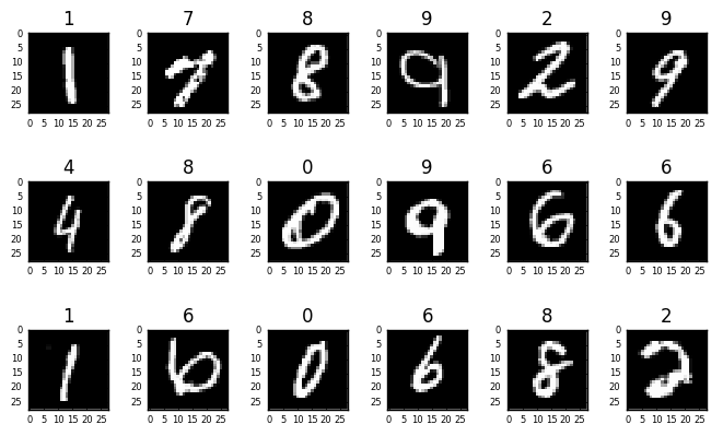
So our network succeeds in 96% of our test data. Let's draw 24 samples from the 4% which it is missing just for getting an idea why it fails to recognize these samples.
print(missed[0:24])
plt.rcParams['figure.figsize'] = (8,6)
for i in range(0, 24):
    plt.subplot(4, 6, i+1)
    img = mnist.test.images[missed[i]].reshape(28,28)
    true_label = mnist.test.labels[missed[i]].argmax()
    pred_label = y_pred[missed[i]].argmax()
    plt.imshow(img, cmap='gray', interpolation='none')
    title = "t:%s, p:%s" % (true_label, pred_label)
    plt.title(title, fontsize=11)
    plt.subplots_adjust(hspace=0.0, wspace=0.5)
    plt.axis('off')

By looking at these samples, it's understandable why in some cases it's easy to confuse between digits. Even humans can make similar confusions. However, we can improve our network by adding more hidden layers, or choosing better activation functions. This could be a nice idea for a course project ...
Course Project 1
In previous course units we have covered the following computer vision test cases:
In all these three cases we have used CNN's (Convolutional Neural Networks). Can we solve these cases with RNN's? If yes, can we do better in terms of accuracy, model size, and computational speed? Perform an exhaustive analysis and write a detailed report.
Course Project 3
Go over the IMDb sentiment analysis test case and see if it can be handled better by an RNN.