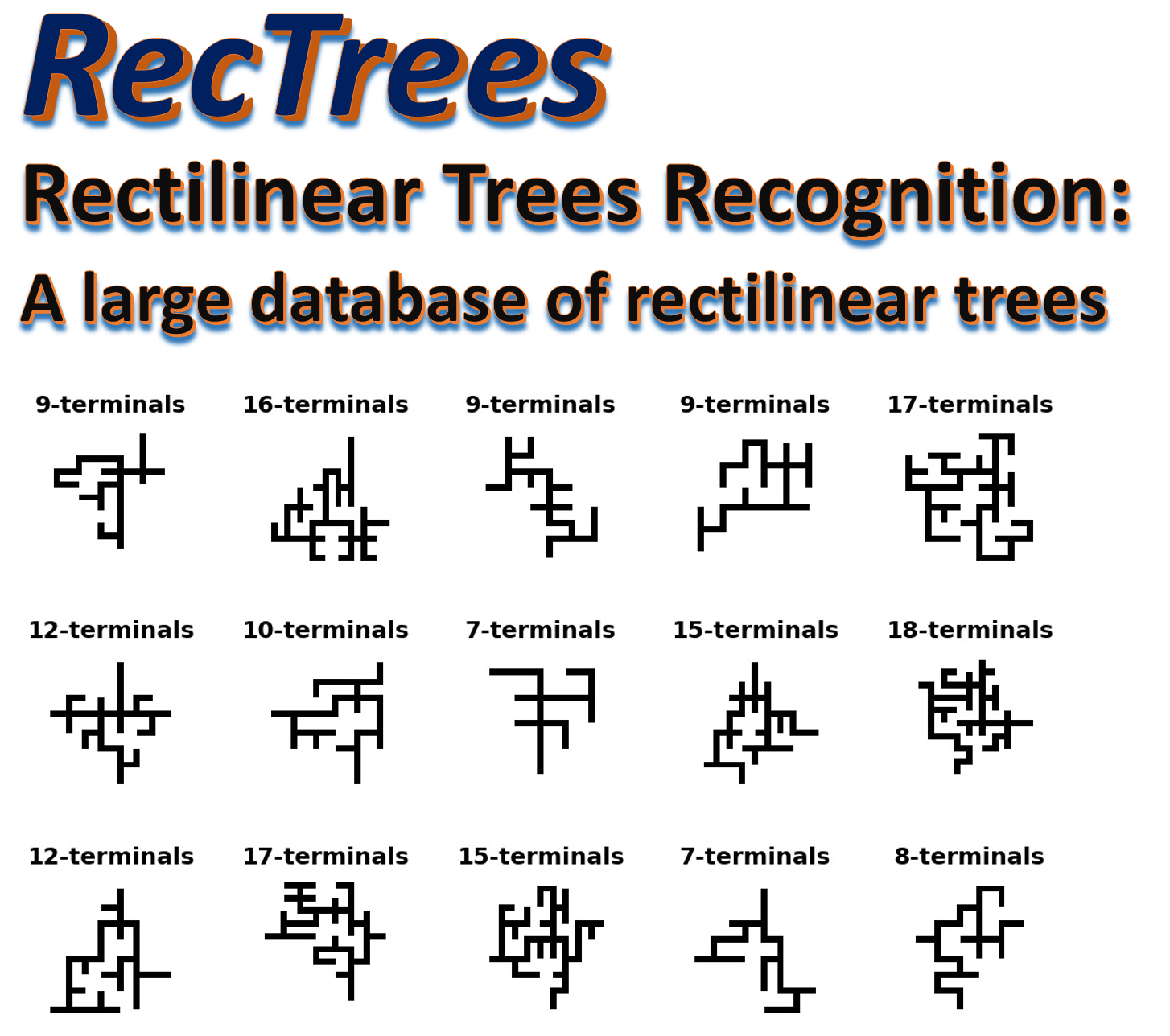
RecTrees is a large data set of simple 48x48 pixels black and white images of rectlinear tree routings. Rectlinear trees are frequently used in electronics VLSI domains for connecting electronic units (sometimes called Steiner Trees). At post slicon stages, sometimes automatic optical recognition methods are needed to examine defective units. We therefore believe that Neural networks for visual recognition can be very helpful in the chip layout design domain. However, this ipython notebook is intended as basic study unit in the deep leaarning field, that covers simple recognition tasks that can be used in the class room, lab exercises, and in final course projects. At the end of the notebook we will portray a more advanced topics that can be pursued for research and practical applications. As can be seen from the above diagram, these types of images are pretty simple and concise. There are no angles or gray pixels in these images, only black and white pixels, and only straight lines that are either vertical or horizontal. As such, we expect that it would not be hard to devise neural networks that can detect the following feature

How many terminal vertices a rectree has?
A terminal is simply a point of degree 1 (has only one edge). Sometimes also called a leaf node in graphs theory.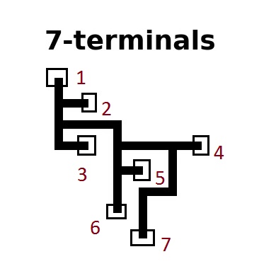
How many edges the tree has?
How many corner points a tree has?
A corner is simply a junction point in which two edges meet orthogonally.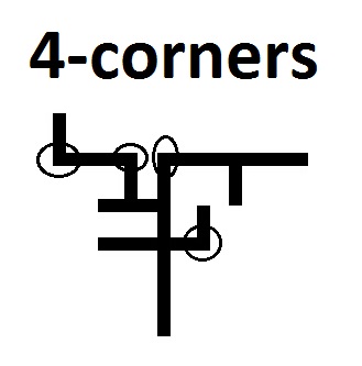

The RecTrees database consists of half million black/white 48x48 pixesl images of rectilinear trees. They were generated by an automatic Networkx Python script with random graphs. To make it as simple as possible, we used grayscale 48x48 pixels images, so that it can be processed by standard pc systems with modest computing resources. It is intented to serve as a simple and clean data set for preliminary excursions, tutorials, or course projects in deep learning courses.

It is also intended to serve as a clear and simple minded data set for benchmarking deep learning libraries and deep learning hardware (like GPU systems). As far as we tried within the Keras library, achieving high accuracy prediction scores does require a non-trivial effort and compute time. It is also our hope that this large database of trees can be used for more advanced research on applying deep learning techniques in the VLSI layout domain.

The RecTrees data set consists of 10 HDF5 files, each contains 50000 48x48 pixels grayscale images. So in total, we have 500,000 48x48 grayscale images. We believe that 50K images are sufficient for training (at least for simple tasks as terminals and edge counting). So you may not need to download all the data sets.

Depending on the classification problem you want to solve, you may need to apply some scripts in order to extract a balanced subset from these data sets.

You will need to install the h5py Python module. Reading and writing HDF5 files can be easily learned from the following tutorial: https://www.getdatajoy.com/learn/Read_and_Write_HDF5_from_Python

Some Python utilities for manipulating these data sets can be found here:
http://www.samyzaf.com/cgi-bin/view_file.py?file=ML/rectrees/rectrees.py
This module contains utilities for iterating over the images and graphs within each of the above HDF5 archives, and utilities for querying or manipulating graphs and trees. They are base on the Python Networkx module, which you may need to install before using them.

Prerequisites¶

The code for this IPython notebook was tested on Windows 10, Python 2.7 with keras, numpy, matplotlib and jupyter. The deep learning hardware we used was an NVIDIA GPU (GeForce GTX950) with cuDNN version 5103. Of course, it can also be run on CPU but it will be significantly slower (not recommended).

To run the code in this notebook, you'll also need to download a few private libraries which we use in other examples of this course:

Here are the Python modules and basic definitions that we need in this project

from keras.models import Sequential, load_model
from keras.layers import Dense, Dropout, Activation, Flatten
from keras.layers import Convolution2D, MaxPooling2D, AveragePooling2D, ZeroPadding2D
from keras.optimizers import SGD
from keras.utils import np_utils
from keras.layers.advanced_activations import SReLU, ELU, LeakyReLU
from keras.utils.visualize_util import plot
import matplotlib.pyplot as plt
import matplotlib.cm
from kerutils import *
from imgutils import *
%matplotlib inline

#classes = range(7,19)
classes = range(0,12)
class_name = dict((i, '%d-terminals' % (7+i,)) for i in classes)
nb_classes = len(class_name)

Using Theano backend.
DEBUG: nvcc STDOUT mod.cu
   Creating library C:/Users/samy/AppData/Local/Theano/compiledir_Windows-10-10.0.14393-Intel64_Family_6_Model_94_Stepping_3_GenuineIntel-2.7.11-64/tmpr5vbk2/265abc51f7c376c224983485238ff1a5.lib and object C:/Users/samy/AppData/Local/Theano/compiledir_Windows-10-10.0.14393-Intel64_Family_6_Model_94_Stepping_3_GenuineIntel-2.7.11-64/tmpr5vbk2/265abc51f7c376c224983485238ff1a5.exp

Using gpu device 0: GeForce GTX 950 (CNMeM is enabled with initial size: 80.0% of memory, cuDNN 5103)
c:\anaconda2\lib\site-packages\theano\sandbox\cuda\__init__.py:600: UserWarning: Your cuDNN version is more recent than the one Theano officially supports. If you see any problems, try updating Theano or downgrading cuDNN to version 5.
  warnings.warn(warn)

# These are css/html styles for good looking ipython notebooks
from IPython.core.display import HTML
css = open('style-notebook.css').read()
HTML('<style>{}</style>'.format(css));

Terminals Counting Challenge¶

A simple example to start with is to build a neural network for recognizing the number of terminals. The network accepts as inputs 48x48 images of rectilinear trees and outputs their terminal numbers.

Preparing training and validation data sets¶

The archived data sets above contains half million rectilinear trees, which is too big for our first exercise. We will start with a small subset of 24000 training samples, 2000 samples from each group of 7-treminals, 8-terminals, ..., 18-terminals (12 groups). And a small validation set of 6000 samples (500 from each group). We have completely ignored rectilinear trees with less than 7 terminals, since there are not many of them and thus including them could turn our training set imbalanced. We therefor use class number 0 for trees with 7-terminals, class number 1 for trees with 8-terminals, etc...

Preparing such balanced subset requires that you iterate over the large data sets and pick the right number of trees for each type. Here are our training and validation sets:

so we suggest that you start with a smaller data sets first, and later increase their size if needed. You can create your own training and validation sets by applying utilities from the modules rectrees and imgutils.

Load training and test data¶

The imgutils module also contains a utility load_data for loading HDF5 files to memory (as Numpy arrays). This method accepts the names of your training and validation data set files, and it returns the following six Numpy arrays:

X_train: an array of 24000 images whose shape is 24000x48x48.
y_train: a one dimensional array of 24000 integers representing the class number of each image in X_train.
Y_train: an 24000 array of one-hot vectors needed for Keras model. For more details see: http://stackoverflow.com/questions/29831489/numpy-1-hot-array
X_test: an array of 6000 validation images (6000x48x48)
y_test: validation class array
Y_test: one-hot vectors for the validation samples

It should be noted that in addition to reading the images from the HDF5 file, the load_data method also performs some normalization of the image data like scaling it to a unit interval and centering it around the mean value. You can control these actions by additional optional arguments of this command. Please look at the source code to learn more.

X_train, y_train, Y_train, X_test, y_test, Y_test = load_data('train.h5', 'test.h5')

print('X_train shape:', X_train.shape)
print(X_train.shape[0], 'training samples')
print(X_test.shape[0], 'validation samples')

Loading training data set: train.h5
Total num images in file: 24000
Load progress: 100%   
Time: 9.69 seconds
Loading validation data set: test.h5
Total num images in file: 4800
Load progress: 100%   
Time: 2.37 seconds
24000 training samples
4800 validation samples
Image shape: (48L, 48L, 1L)
X_train shape: (24000L, 48L, 48L, 1L)
24000 training samples
4800 validation samples

Let's also write two small utilities for drawing samples of images, so we can inspect our results visually.

def draw_image(img, id):
    img = img.reshape(48,48)
    plt.imshow(img, cmap='gray', interpolation='none')
    plt.title("%d: %s" % (id, class_name[id]), fontsize=15, fontweight='bold', y=1.08)
    plt.axis('off')
    plt.show()

Let's draw image 18 in the X_train array as example

draw_image(X_train[18], y_train[18])

As we can see, the image is a bit blurry due to the normalization procedures that the load_data method has done to the original data. If you want to draw the raw data as it is in the HDF5 file, use the h5_get method to extract the raw image from the HDF5 file directly:

img = h5_get('train.h5', 'img_18')
id = y_train[18]
draw_image(img, id)

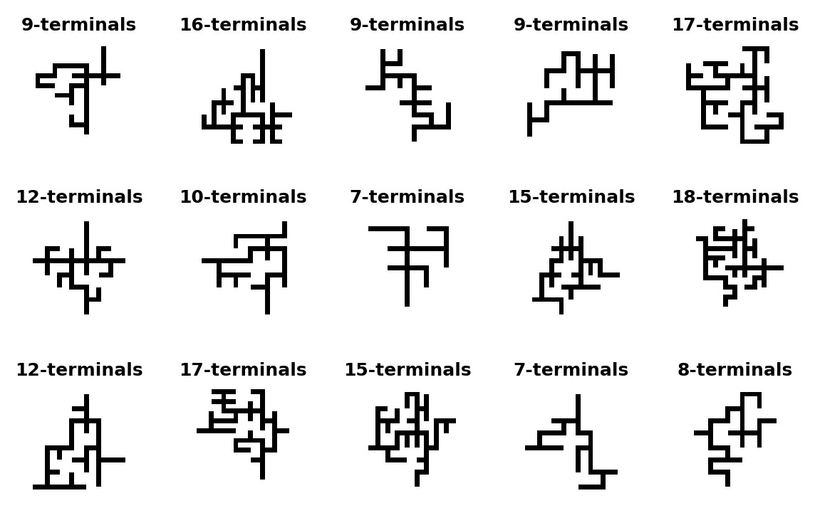
Sometimes we want to inspect a larger group of images in parallel, so we also provide a method for drawing a grid of consecutive images.

def draw_sample(X, y, n, rows=4, cols=4, imfile=None, fontsize=9):
    for i in range(0, rows*cols):
        plt.subplot(rows, cols, i+1)
        img = X[n+i].reshape(48,48)
        plt.imshow(img, cmap='gray', interpolation='none')
        id = y[n+i]
        plt.title("%d: %s" % (id, class_name[id]), fontsize=fontsize, y=1.08)
        plt.axis('off')
        plt.subplots_adjust(wspace=0.8, hspace=0.1)

draw_sample(X_train, y_train, 400, 3, 5)

Again, ignore the blurring images due to image normalization. The original images are pure black and white of course.

Counting terminals in RecTrees¶

Let's start with the terminals counting problem. Our aim is to build a neural network which accepts 48x48 grayscale image of a rectilinear tree and outputs the number of of terminals this tree has.

We start with a simple Keras model which combines one Convolution2D layer with two Dense layers. Although simple in terms of code, it is too expensive in terms of computation and hardware, as it contains 70 million parameters! This is way too much and should be avoided in general. However, we want to experiment with the common use of Dense layers and see why they are not good for image processing. In general, Dense layers should be avoided as much as possible when dealing with image data. The general practice is to use Convolution and Pooling layers. These two types of layers are explained in more detail in the following two articles, which we recommend to read before you approach the following code:

A Neural Network for counting terminals in RecTrees¶

Let's start with the terminals counting problem. Our aim is to build a nueral network which accepts 48x48 grayscale image of a rectilinear tree and outputs the number of of terminals this tree has.

We start with a simple Keras model which combines one Convolution2D layer and two Dense layers. Although simple in terms of code, it is too expensive in terms of computation and hardware, as it contains 70 million parameters! This is way too much and should be avoided in general. However, we want to experiment with the common use of Dense layers and see why they are not good for image processing. In general, Dense layers should be avoided as much as possible when dealing with image data. The general practice is to use Convolution and Pooling layers. These two types of layers are explained in more detail in the following two articles, which we recommend to read before you approach the following code:

Lets Train Model 1¶

We now define our first model for the recognizing the number of terminals in RecTrees. Note that unlike the common practice, we decided to use the SReLU activation method instead of the more popular relu activation. We did several test with relu but SReLU seems to be more appropriate for RecTrees. One of the amazing facts about SReLU is that it adapts itself during the learning process and not a constant function as other activations. You may read more about it in the following papers:

nb_epoch = 100
batch_size = 32
input_shape = X_train.shape[1:]

model = Sequential(name="model_1")
model.add(Convolution2D(64, 3, 3, input_shape=input_shape))
model.add(SReLU())

model.add(Flatten())

model.add(Dense(512))
model.add(SReLU())
model.add(Dropout(0.4))

model.add(Dense(256))
model.add(SReLU())
model.add(Dropout(0.4))

model.add(Dense(nb_classes))
model.add(Activation('softmax'))

print(model.summary())
save_model_summary(model, "model_1_summary.txt")
write_file("model_1.json", model.to_json())
fmon = FitMonitor(thresh=0.09, minacc=0.999, filename="model_1_autosave.h5")

model.compile(optimizer='adam', loss='categorical_crossentropy', metrics=['accuracy'])

hist = model.fit(
    X_train,
    Y_train,
    batch_size=batch_size,
    nb_epoch=nb_epoch,
    shuffle=True,
    validation_data=(X_test, Y_test),
    verbose=0,
    callbacks = [fmon]
)

model_file = "model_1.h5"
print("Saving model to:", model_file)
model.save(model_file)
plot(model, to_file="model_1_scheme.png", show_layer_names=False, show_shapes=True)

show_scores(model, hist, X_train, Y_train, X_test, Y_test)

____________________________________________________________________________________________________
Layer (type)                     Output Shape          Param #     Connected to                     
====================================================================================================
convolution2d_1 (Convolution2D)  (None, 46L, 46L, 64)  640         convolution2d_input_1[0][0]      
____________________________________________________________________________________________________
srelu_1 (SReLU)                  (None, 46L, 46L, 64)  541696      convolution2d_1[0][0]            
____________________________________________________________________________________________________
flatten_1 (Flatten)              (None, 135424)        0           srelu_1[0][0]                    
____________________________________________________________________________________________________
dense_1 (Dense)                  (None, 512)           69337600    flatten_1[0][0]                  
____________________________________________________________________________________________________
srelu_2 (SReLU)                  (None, 512)           2048        dense_1[0][0]                    
____________________________________________________________________________________________________
dropout_1 (Dropout)              (None, 512)           0           srelu_2[0][0]                    
____________________________________________________________________________________________________
dense_2 (Dense)                  (None, 256)           131328      dropout_1[0][0]                  
____________________________________________________________________________________________________
srelu_3 (SReLU)                  (None, 256)           1024        dense_2[0][0]                    
____________________________________________________________________________________________________
dropout_2 (Dropout)              (None, 256)           0           srelu_3[0][0]                    
____________________________________________________________________________________________________
dense_3 (Dense)                  (None, 12)            3084        dropout_2[0][0]                  
____________________________________________________________________________________________________
activation_1 (Activation)        (None, 12)            0           dense_3[0][0]                    
====================================================================================================
Total params: 70,017,420
Trainable params: 70,017,420
Non-trainable params: 0
____________________________________________________________________________________________________
None
Train begin: 2017-01-01 19:52:43
Stop file: stop_training_file.keras (create this file to stop training gracefully)
Pause file: pause_training_file.keras (create this file to pause training and view graphs)
batch_size = 32
do_validation = True
metrics = ['loss', 'acc', 'val_loss', 'val_acc']
nb_epoch = 100
nb_sample = 24000
verbose = 0
.....05% epoch=5, acc=0.568542, loss=0.971951, val_acc=0.663333, val_loss=0.849731, time=0.115 hours
.....10% epoch=10, acc=0.678792, loss=0.748152, val_acc=0.707917, val_loss=0.756233, time=0.211 hours
.....15% epoch=15, acc=0.755167, loss=0.587179, val_acc=0.741042, val_loss=0.718850, time=0.307 hours
.....20% epoch=20, acc=0.804958, loss=0.492191, val_acc=0.779375, val_loss=0.681137, time=0.403 hours
.....25% epoch=25, acc=0.832708, loss=0.426067, val_acc=0.695625, val_loss=0.897914, time=0.499 hours
.....30% epoch=30, acc=0.867083, loss=0.357213, val_acc=0.779375, val_loss=0.752492, time=0.595 hours
.....35% epoch=35, acc=0.885083, loss=0.309000, val_acc=0.781458, val_loss=0.770379, time=0.690 hours
.....40% epoch=40, acc=0.901667, loss=0.273201, val_acc=0.773333, val_loss=0.820073, time=0.785 hours
.....45% epoch=45, acc=0.904708, loss=0.259520, val_acc=0.770625, val_loss=0.854607, time=0.881 hours
.....50% epoch=50, acc=0.913750, loss=0.246238, val_acc=0.758958, val_loss=0.983357, time=0.976 hours
.....55% epoch=55, acc=0.917042, loss=0.234406, val_acc=0.775625, val_loss=0.863706, time=1.071 hours
.....60% epoch=60, acc=0.923917, loss=0.213466, val_acc=0.765833, val_loss=0.949016, time=1.167 hours
.....65% epoch=65, acc=0.925167, loss=0.211941, val_acc=0.746042, val_loss=1.017067, time=1.262 hours
.....70% epoch=70, acc=0.930042, loss=0.193352, val_acc=0.715833, val_loss=1.241069, time=1.357 hours
.....75% epoch=75, acc=0.940375, loss=0.178771, val_acc=0.748958, val_loss=1.100173, time=1.453 hours
.....80% epoch=80, acc=0.937750, loss=0.183755, val_acc=0.772917, val_loss=1.085037, time=1.548 hours
.....85% epoch=85, acc=0.945250, loss=0.156339, val_acc=0.740000, val_loss=1.149049, time=1.643 hours
.....90% epoch=90, acc=0.947125, loss=0.153056, val_acc=0.763125, val_loss=1.167173, time=1.739 hours
.....95% epoch=95, acc=0.950583, loss=0.145004, val_acc=0.754792, val_loss=1.221379, time=1.834 hours
.... 99% epoch=99 acc=0.954042 loss=0.134188
Train end: 2017-01-01 21:47:21
Total run time: 1.910 hours
max_acc = 0.954042  epoch = 99
max_val_acc = 0.797083  epoch = 27
No checkpoint model found.
Saving model to: model_1.h5
Training: accuracy   = 0.999042 loss = 0.007824
Validation: accuracy = 0.770625 loss = 1.126207
Over fitting score   = 0.162030
Under fitting score  = 0.132790
Params count: 70017420
stop epoch = 99
nb_epoch = 100
batch_size = 32
nb_sample = 24000

loss, accuracy = model.evaluate(X_train, Y_train, verbose=0)
print("Training: accuracy = %f  ;  loss = %f" % (accuracy, loss))

Training: accuracy = 0.998500  ;  loss = 0.009213

loss, accuracy = model.evaluate(X_test, Y_test, verbose=0)
print("Validation: accuracy1 = %f  ;  loss1 = %f" % (accuracy, loss))

Validation: accuracy1 = 0.895625  ;  loss1 = 1.100054

Although the training accuracy is quite high (99.9% !), the overall result is not good! The 12% gap with respect to the validation accuracy is an alarming indication of overfitting (which is also clearly noticeable from the accuracy and loss graphs above). Our model is successful on the training set only and is not as successful for any other data.

Inspecting the output¶

Befor we search for a new model, let's take a quick look on some of the cases that our model missed. It may give us clues on the strengths and weaknesses of NN models, and what we can expect from these artificial models.

The predict_classes method is helpful for getting a vector (y_pred) of the predicted classes of our model 1. We should compare y_pred to the expected true classes y_test in order to get the false cases:

y_pred = model.predict_classes(X_test)

4800/4800 [==============================] - 2s

true_preds = [(x,y) for (x,y,p) in zip(X_test, y_test, y_pred) if y == p]
false_preds = [(x,y,p) for (x,y,p) in zip(X_test, y_test, y_pred) if y != p]
print("Number of valid predictions: ", len(true_preds))
print("Number of invalid predictions:", len(false_preds))

Number of valid predictions:  3699
Number of invalid predictions: 1101

The array false_preds consists of all triples (x,y,p) where x is an image, y is its true class, and p is the false predicted value of model.

Lets visualize a sample of 15 items:

for i,(x,y,p) in enumerate(false_preds[0:15]):
    plt.subplot(3, 5, i+1)
    img = x.reshape(48,48)
    plt.imshow(img, cmap='gray')
    plt.title("%d\ny: %s\np: %s" % (i, class_name[y], class_name[p]), fontsize=9, loc='left')
    plt.axis('off')
    plt.subplots_adjust(wspace=1.0, hspace=0.7)

Interestingly, in all the observed 15 cases, our model missed the correct answer by one terminal only, which is not so bad. Almost a human behavior (in fact when I try to count the number of terminals manualy, I sometimes miss by 2 or even by 3!)

Second Keras Model for the RecTrees database¶

Lets try to add an additional Convolution2D layer and reduce the width of the Dense layers. The number of parameters is still too high (32 millions), but much less than model 1.

nb_epoch = 100
batch_size = 32
input_shape = X_train.shape[1:]

model = Sequential(name="model_2")
model.add(Convolution2D(64, 3, 3, input_shape=input_shape))
model.add(SReLU())

model.add(Convolution2D(64, 3, 3, input_shape=input_shape))
model.add(SReLU())

model.add(Flatten())

model.add(Dense(256))
model.add(SReLU())
model.add(Dropout(0.4))

model.add(Dense(64))
model.add(SReLU())
model.add(Dropout(0.4))

model.add(Dense(nb_classes))
model.add(Activation('softmax'))

print(model.summary())
save_model_summary(model, "model_2_summary.txt")
write_file("model_2.json", model.to_json())
fmon = FitMonitor(thresh=0.09, minacc=0.999, filename="model_2_autosave.h5")

model.compile(optimizer='adam', loss='categorical_crossentropy', metrics=['accuracy'])

hist = model.fit(
    X_train,
    Y_train,
    batch_size=batch_size,
    nb_epoch=nb_epoch,
    shuffle=True,
    validation_data=(X_test, Y_test),
    verbose=0,
    callbacks = [fmon]
)

model_file = "model_2.h5"
print("Saving model to:", model_file)
model.save(model_file)
plot(model, to_file="model_2_scheme.png", show_layer_names=False, show_shapes=True)

show_scores(model, hist, X_train, Y_train, X_test, Y_test)

____________________________________________________________________________________________________
Layer (type)                     Output Shape          Param #     Connected to                     
====================================================================================================
convolution2d_2 (Convolution2D)  (None, 46L, 46L, 64)  640         convolution2d_input_2[0][0]      
____________________________________________________________________________________________________
srelu_4 (SReLU)                  (None, 46L, 46L, 64)  541696      convolution2d_2[0][0]            
____________________________________________________________________________________________________
convolution2d_3 (Convolution2D)  (None, 44L, 44L, 64)  36928       srelu_4[0][0]                    
____________________________________________________________________________________________________
srelu_5 (SReLU)                  (None, 44L, 44L, 64)  495616      convolution2d_3[0][0]            
____________________________________________________________________________________________________
flatten_2 (Flatten)              (None, 123904)        0           srelu_5[0][0]                    
____________________________________________________________________________________________________
dense_4 (Dense)                  (None, 256)           31719680    flatten_2[0][0]                  
____________________________________________________________________________________________________
srelu_6 (SReLU)                  (None, 256)           1024        dense_4[0][0]                    
____________________________________________________________________________________________________
dropout_3 (Dropout)              (None, 256)           0           srelu_6[0][0]                    
____________________________________________________________________________________________________
dense_5 (Dense)                  (None, 64)            16448       dropout_3[0][0]                  
____________________________________________________________________________________________________
srelu_7 (SReLU)                  (None, 64)            256         dense_5[0][0]                    
____________________________________________________________________________________________________
dropout_4 (Dropout)              (None, 64)            0           srelu_7[0][0]                    
____________________________________________________________________________________________________
dense_6 (Dense)                  (None, 12)            780         dropout_4[0][0]                  
____________________________________________________________________________________________________
activation_2 (Activation)        (None, 12)            0           dense_6[0][0]                    
====================================================================================================
Total params: 32,813,068
Trainable params: 32,813,068
Non-trainable params: 0
____________________________________________________________________________________________________
None
Train begin: 2017-01-01 22:46:24
Stop file: stop_training_file.keras (create this file to stop training gracefully)
Pause file: pause_training_file.keras (create this file to pause training and view graphs)
batch_size = 32
do_validation = True
metrics = ['loss', 'acc', 'val_loss', 'val_acc']
nb_epoch = 100
nb_sample = 24000
verbose = 0
.....05% epoch=5, acc=0.775500, loss=0.544670, val_acc=0.920833, val_loss=0.278887, time=0.228 hours
.....10% epoch=10, acc=0.872583, loss=0.339086, val_acc=0.955625, val_loss=0.150487, time=0.417 hours
.....15% epoch=15, acc=0.902083, loss=0.268637, val_acc=0.972083, val_loss=0.094276, time=0.606 hours
.....20% epoch=20, acc=0.916792, loss=0.234706, val_acc=0.961875, val_loss=0.113011, time=0.795 hours
.....25% epoch=25, acc=0.928000, loss=0.205397, val_acc=0.979375, val_loss=0.084526, time=0.984 hours
.....30% epoch=30, acc=0.936417, loss=0.184584, val_acc=0.980833, val_loss=0.060914, time=1.173 hours
.....35% epoch=35, acc=0.952375, loss=0.142559, val_acc=0.981042, val_loss=0.067010, time=1.361 hours
.....40% epoch=40, acc=0.954542, loss=0.134788, val_acc=0.979792, val_loss=0.076306, time=1.549 hours
.....45% epoch=45, acc=0.955917, loss=0.132472, val_acc=0.987292, val_loss=0.057707, time=1.738 hours
.....50% epoch=50, acc=0.958250, loss=0.131790, val_acc=0.985417, val_loss=0.057163, time=1.928 hours
.....55% epoch=55, acc=0.960333, loss=0.118335, val_acc=0.980833, val_loss=0.071680, time=2.117 hours
.....60% epoch=60, acc=0.965625, loss=0.103045, val_acc=0.987708, val_loss=0.054723, time=2.306 hours
.....65% epoch=65, acc=0.959833, loss=0.124831, val_acc=0.980208, val_loss=0.067420, time=2.496 hours
.....70% epoch=70, acc=0.967875, loss=0.101036, val_acc=0.974167, val_loss=0.097241, time=2.686 hours
.....75% epoch=75, acc=0.963542, loss=0.110849, val_acc=0.937292, val_loss=0.205707, time=2.878 hours
.....80% epoch=80, acc=0.964750, loss=0.111151, val_acc=0.981250, val_loss=0.079582, time=3.069 hours
.....85% epoch=85, acc=0.960708, loss=0.124320, val_acc=0.973750, val_loss=0.112609, time=3.259 hours
.....90% epoch=90, acc=0.956292, loss=0.137532, val_acc=0.975000, val_loss=0.079073, time=3.449 hours
.....95% epoch=95, acc=0.962583, loss=0.119837, val_acc=0.976875, val_loss=0.098852, time=3.639 hours
.... 99% epoch=99 acc=0.959708 loss=0.124383
Train end: 2017-01-02 02:33:49
Total run time: 3.790 hours
max_acc = 0.973833  epoch = 82
max_val_acc = 0.990833  epoch = 76
No checkpoint model found.
Saving model to: model_2.h5
Training: accuracy   = 0.994625 loss = 0.018825
Validation: accuracy = 0.975625 loss = 0.096358
Over fitting score   = 0.022391
Under fitting score  = 0.037299
Params count: 32813068
stop epoch = 99
nb_epoch = 100
batch_size = 32
nb_sample = 24000

Seems like the second Convolution layer that we added has drastically reduced overfitting from over 12% to less than 2%! This is also clearly displayed in the accracy and loss graphs above. The two graphs are tightly closed. But of course there's still room for improvement.

Model 3¶

We will add a third Convolution layer, and increase the filter size to 5x5 in the first two layers. In adition, we add three new MaxPooling2D layers (one after each Convolution2D). The immediate effect of these layers is a drastic reduction in the model number of parameters from 90 million to 915K almost 1% compared to model 1. Even if we get similar results to model 1, it would be considered a success and a proof for why Convolution and Pooling layers are the right kind of layers to use for image data.

nb_epoch = 100
batch_size = 32
input_shape = X_train.shape[1:]

model = Sequential(name="model_3")
model.add(Convolution2D(64, 5, 5, input_shape=input_shape))
model.add(SReLU())

model.add(MaxPooling2D(pool_size=(2, 2)))

model.add(Convolution2D(64, 5, 5, input_shape=input_shape))
model.add(SReLU())

model.add(MaxPooling2D(pool_size=(2, 2)))

model.add(Convolution2D(64, 3, 3, input_shape=input_shape))
model.add(SReLU())

model.add(MaxPooling2D(pool_size=(2, 2)))

model.add(Flatten())

model.add(Dense(256))
model.add(SReLU())
model.add(Dropout(0.5))

model.add(Dense(128))
model.add(SReLU())
model.add(Dropout(0.5))

model.add(Dense(nb_classes))
model.add(Activation('softmax'))

print(model.summary())
save_model_summary(model, "model_3_summary.txt")
write_file("model_3.json", model.to_json())
fmon = FitMonitor(thresh=0.09, minacc=0.999, filename="model_3_autosave.h5")

model.compile(optimizer='adam', loss='categorical_crossentropy', metrics=['accuracy'])

hist = model.fit(
    X_train,
    Y_train,
    batch_size=batch_size,
    nb_epoch=nb_epoch,
    shuffle=True,
    validation_data=(X_test, Y_test),
    verbose=0,
    callbacks = [fmon]
)

model_file = "model_3.h5"
print("Saving model to:", model_file)
model.save(model_file)
plot(model, to_file="model_3_scheme.png", show_layer_names=False, show_shapes=True)

show_scores(model, hist, X_train, Y_train, X_test, Y_test)

____________________________________________________________________________________________________
Layer (type)                     Output Shape          Param #     Connected to                     
====================================================================================================
convolution2d_1 (Convolution2D)  (None, 44L, 44L, 64)  1664        convolution2d_input_1[0][0]      
____________________________________________________________________________________________________
srelu_1 (SReLU)                  (None, 44L, 44L, 64)  495616      convolution2d_1[0][0]            
____________________________________________________________________________________________________
maxpooling2d_1 (MaxPooling2D)    (None, 22L, 22L, 64)  0           srelu_1[0][0]                    
____________________________________________________________________________________________________
convolution2d_2 (Convolution2D)  (None, 18L, 18L, 64)  102464      maxpooling2d_1[0][0]             
____________________________________________________________________________________________________
srelu_2 (SReLU)                  (None, 18L, 18L, 64)  82944       convolution2d_2[0][0]            
____________________________________________________________________________________________________
maxpooling2d_2 (MaxPooling2D)    (None, 9L, 9L, 64)    0           srelu_2[0][0]                    
____________________________________________________________________________________________________
convolution2d_3 (Convolution2D)  (None, 7L, 7L, 64)    36928       maxpooling2d_2[0][0]             
____________________________________________________________________________________________________
srelu_3 (SReLU)                  (None, 7L, 7L, 64)    12544       convolution2d_3[0][0]            
____________________________________________________________________________________________________
maxpooling2d_3 (MaxPooling2D)    (None, 3L, 3L, 64)    0           srelu_3[0][0]                    
____________________________________________________________________________________________________
flatten_1 (Flatten)              (None, 576)           0           maxpooling2d_3[0][0]             
____________________________________________________________________________________________________
dense_1 (Dense)                  (None, 256)           147712      flatten_1[0][0]                  
____________________________________________________________________________________________________
srelu_4 (SReLU)                  (None, 256)           1024        dense_1[0][0]                    
____________________________________________________________________________________________________
dropout_1 (Dropout)              (None, 256)           0           srelu_4[0][0]                    
____________________________________________________________________________________________________
dense_2 (Dense)                  (None, 128)           32896       dropout_1[0][0]                  
____________________________________________________________________________________________________
srelu_5 (SReLU)                  (None, 128)           512         dense_2[0][0]                    
____________________________________________________________________________________________________
dropout_2 (Dropout)              (None, 128)           0           srelu_5[0][0]                    
____________________________________________________________________________________________________
dense_3 (Dense)                  (None, 12)            1548        dropout_2[0][0]                  
____________________________________________________________________________________________________
activation_1 (Activation)        (None, 12)            0           dense_3[0][0]                    
====================================================================================================
Total params: 915,852
Trainable params: 915,852
Non-trainable params: 0
____________________________________________________________________________________________________
None

DEBUG: nvcc STDOUT mod.cu
   Creating library C:/Users/samy/AppData/Local/Theano/compiledir_Windows-10-10.0.14393-Intel64_Family_6_Model_94_Stepping_3_GenuineIntel-2.7.11-64/tmp_wypmf/8e7d60a6808914f8d433e5bd84cf0019.lib and object C:/Users/samy/AppData/Local/Theano/compiledir_Windows-10-10.0.14393-Intel64_Family_6_Model_94_Stepping_3_GenuineIntel-2.7.11-64/tmp_wypmf/8e7d60a6808914f8d433e5bd84cf0019.exp

DEBUG: nvcc STDOUT mod.cu
   Creating library C:/Users/samy/AppData/Local/Theano/compiledir_Windows-10-10.0.14393-Intel64_Family_6_Model_94_Stepping_3_GenuineIntel-2.7.11-64/tmp09ib5u/b9688604acbcfcdd45ccf1c9bd8114a4.lib and object C:/Users/samy/AppData/Local/Theano/compiledir_Windows-10-10.0.14393-Intel64_Family_6_Model_94_Stepping_3_GenuineIntel-2.7.11-64/tmp09ib5u/b9688604acbcfcdd45ccf1c9bd8114a4.exp

Train begin: 2017-01-02 12:04:28
Stop file: stop_training_file.keras (create this file to stop training gracefully)
Pause file: pause_training_file.keras (create this file to pause training and view graphs)
batch_size = 32
do_validation = True
metrics = ['loss', 'acc', 'val_loss', 'val_acc']
nb_epoch = 100
nb_sample = 24000
verbose = 0
.....05% epoch=5, acc=0.845125, loss=0.392574, val_acc=0.946250, val_loss=0.191832, time=0.068 hours
.....10% epoch=10, acc=0.910333, loss=0.242289, val_acc=0.956458, val_loss=0.123774, time=0.125 hours
.....15% epoch=15, acc=0.929417, loss=0.197352, val_acc=0.975833, val_loss=0.073973, time=0.182 hours
.....20% epoch=20, acc=0.944417, loss=0.156441, val_acc=0.953542, val_loss=0.153584, time=0.239 hours
.....25% epoch=25, acc=0.948667, loss=0.150141, val_acc=0.974167, val_loss=0.093788, time=0.297 hours
.....30% epoch=30, acc=0.947125, loss=0.162347, val_acc=0.973750, val_loss=0.079984, time=0.354 hours
.....35% epoch=35, acc=0.956792, loss=0.130196, val_acc=0.985208, val_loss=0.056711, time=0.411 hours
.....40% epoch=40, acc=0.963750, loss=0.113933, val_acc=0.985833, val_loss=0.056117, time=0.468 hours
.....45% epoch=45, acc=0.967917, loss=0.117074, val_acc=0.988333, val_loss=0.045027, time=0.525 hours
.....50% epoch=50, acc=0.962583, loss=0.111580, val_acc=0.984375, val_loss=0.056841, time=0.582 hours
.....55% epoch=55, acc=0.962333, loss=0.116465, val_acc=0.988125, val_loss=0.041123, time=0.638 hours
.....60% epoch=60, acc=0.960000, loss=0.118289, val_acc=0.988542, val_loss=0.040611, time=0.695 hours
.....65% epoch=65, acc=0.972417, loss=0.084954, val_acc=0.978125, val_loss=0.068473, time=0.752 hours
.....70% epoch=70, acc=0.974500, loss=0.086902, val_acc=0.984792, val_loss=0.048351, time=0.809 hours
.....75% epoch=75, acc=0.974792, loss=0.080403, val_acc=0.959792, val_loss=0.135975, time=0.865 hours
.....80% epoch=80, acc=0.969292, loss=0.092680, val_acc=0.985833, val_loss=0.051048, time=0.922 hours
.....85% epoch=85, acc=0.975417, loss=0.075875, val_acc=0.987083, val_loss=0.048718, time=0.979 hours
.....90% epoch=90, acc=0.978083, loss=0.075633, val_acc=0.987708, val_loss=0.043128, time=1.036 hours
.....95% epoch=95, acc=0.968458, loss=0.105750, val_acc=0.990625, val_loss=0.035164, time=1.092 hours
.... 99% epoch=99 acc=0.978625 loss=0.064434
Train end: 2017-01-02 13:12:43
Total run time: 1.138 hours
max_acc = 0.987958  epoch = 96
max_val_acc = 0.990625  epoch = 83
No checkpoint model found.
Saving model to: model_3.h5
Training: accuracy   = 0.987042 loss = 0.038440
Validation: accuracy = 0.975833 loss = 0.094004
Over fitting score   = 0.026504
Under fitting score  = 0.035833
Params count: 915852
stop epoch = 99
nb_epoch = 100
batch_size = 32
nb_sample = 24000

loss, accuracy = model.evaluate(X_train, Y_train, verbose=0)
print("Training: accuracy = %f  ;  loss = %f" % (accuracy, loss))

Training: accuracy = 0.987042  ;  loss = 0.038440

loss, accuracy = model.evaluate(X_test, Y_test, verbose=0)
print("Validation: accuracy = %f  ;  loss = %f" % (accuracy, loss))

Validation: accuracy = 0.975833  ;  loss = 0.094004

The training accuracy of model 3 is slightly smaller than in model 2 (by 0.7%) but there are two important factors that make model 3 much better than model 2:

It is a significantly smaller model! only 900K parameters compared to 32 millions parameters in model 2. This is critical.
The correlation between the accuracy and validation graphs is more tight (in spite of the occasional spikes).

With some more fine tuning, we believe that mode 3 can achieve greater accuracy and validation scores, without adding too many parameters. So it is better to invest extra efforts on model 3 rather than model 2 or 1.

We will stop our experiments here and let you try to do better (good luck ;-). Is it possible to achieve 100% accuracy??? And if so, in what cost? We don't want too many parameters (not a fare game!), and we don't want too many layers or too many nuerons. After all we are dealing with a rather simple image database (nice and clean geometrical figures), and we want to replace old school programmers with neural networks ... :-)

You may enlarge your training and validation sets. We used only 24000 training samples. How about using 48000 training samples (4000 per group)? You may also experiment with other activation functions and optimizers (there are plenty of them in Keras). You can also work directly in Theano or TensorFlow.

Before you proceed, lets take a look at some examples in which model 3 fails:

y_pred = model.predict_classes(X_test)

4800/4800 [==============================] - 17s

true_preds = [(x,y) for (x,y,p) in zip(X_test, y_test, y_pred) if y == p]
false_preds = [(x,y,p) for (x,y,p) in zip(X_test, y_test, y_pred) if y != p]
print("Number of valid predictions: ", len(true_preds))
print("Number of invalid predictions:", len(false_preds))

Number of valid predictions:  4684
Number of invalid predictions: 116

Let's draw the first 15 failures

for i,(x,y,p) in enumerate(false_preds[0:15]):
    plt.subplot(3, 5, i+1)
    img = x.reshape(48,48)
    plt.imshow(img, cmap='gray')
    plt.title("%d\ny: %s\np: %s" % (i, class_name[y], class_name[p]), fontsize=9, loc='left')
    plt.axis('off')
    plt.subplots_adjust(wspace=0.8, hspace=0.6)

Again, we see that our model sometimes misses one terminal. Is this the case for all other false predictions? That can be easily checked with the following one line of code

false_preds_2 = [(x,y,p) for (x,y,p) in zip(X_test, y_test, y_pred) if abs(y-p)>=2]

len(false_preds_2)

0

Yep! only 1 terminal missed in all false predictions. It means that a neural network solution is no erratic, and there is hope to close the gap with some additional effort.

Some more challenges¶

You can try counting the number of edges, number of vertices, or the number corners. You will need to generate balanced data sets for these projects (see above). A more interesting challenge would be: can a neural network identify the topological for of a rectilinear tree? The topological form of a given tree T is the "smallest" cannonical tree which is geometrically isomorphic to T. Here are a few examples of trees and their topological forms:

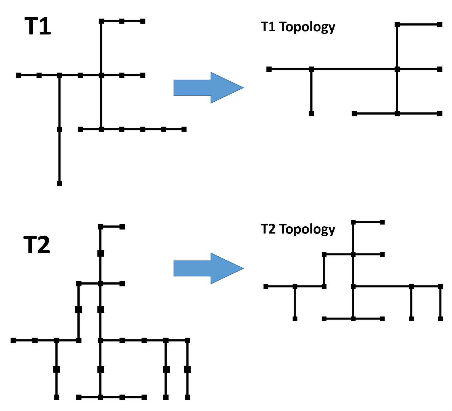
Each topology can be encoded by an integer, and our neural network accepts a 48x48 image of a rectilinear tree and needs to output the integer corresponding to its topology.

The main obstacle we expect in this challenge is creating a large balanced training data set. There are a lot of topologies, and we'll probably need hundreds or maybe thousands sample for each topology, which can make the training set too large. We could restrict ourselves to a small subset of topoloies though. You will also need to mine the half million trees data sets to get enough samples in a balanced state.

Other routing tree properties can be considered for creating similar deep learning challenges. Work in progress ...