VLSI Circuit Open Defects Detection¶

Open defects in VLSI integrated circuit production processes are known to be a common issue. They are usually sought after in the Post Silicon manufacturing stages or when defective chips are returned by customers. Soon after the first wafers come out from the fabrication factories, special test teams are hunting for circuit opens with the aid of highly expensive tester and prober equipments which include high resolution microscopes and cameras that can quickly scan large areas of the chip and produce high quality photos of suspected areas of the chip.

Through the years, VLSI research and development centers introduced advanced methods to process and analyze these photos in order to find defects such as opens or shorts. No doubt that after entering the age of deep learning, there ought to be attempts to attack this problem from the deep learning point of view, which has already proved to be very successful in computer vision.

As this tutorial is intended for a non-expert audience whose main interest is focusing on deep learning with neural networks, we will use a simplistic view of the subject so that we are not distracted from our main interest on showing how deep learning can be applied in the VLSI domain as well as in other domains such as computer vision, natural language processing and so on.

The circuit opens dataset¶

We have generated a simplistic dataset of small defective circuits (due to an open). Each circuit is drawn on a small 48x48 pixels black/white image, and is supposed to contain at least one open defect. The dataset is divided to 5 HDF5 files, each containing 100,000 images. So we have a total of 500,000 images of defective circuits. We hope they are sufficient for training a neural network to do the job (but we must keep a small portion for validation too).

These files can be downloaded from:

For each circuit i, there are 3 entries associated in the dataset:

* img_i - A Numpy matrix for the image itself
* open_i - The open defect rectangular area
* center_i - an (x,y) coordinates of the defect center

Agenda¶

Our aim in this course unit is to suggest a project proposal for applying deep learning methods to VLSI defects detection, based on our simple dataset as a simple example on how to do it. As a student, your goal is to define a deep convolutional neural network that accept a circuit image as input and finds the point in which the circuit is open.

# These are css/html styles for good looking ipython notebooks
from IPython.core.display import HTML
css = open('style-notebook.css').read()
HTML('<style>{}</style>'.format(css))

Feature Information¶

We suggest that a circuit open defect should be coded by a pair of integers which is the coordinate of its center point. This is only a simple suggestion. You may offer a better one if you like. So the features list is the list of all points (i,j) in a 48x48 pixels image space of our circuit.

features = [(i,j) for i in range(48) for j in range(48)]

Here is a simple diagram which explains this idea

Note the Numpy coordinate convention: the first coordinate i designates the row number, the second coordinate j designates the column number. This is also the standard convention in linear algebra matrix notation.

So in total we will have 48x48 features (i.e., 2304 features), which might be too challenging for the training phase. The neural network output layer should have 2304 output neurons, which is a bit discouraging. You may want to refine the list of features by a simple list of regions in which the defect occurs. Once we know the region, it will be easy to locate the defect. Here is an example in which our 48x48 image is divided to 64 6x6 regions

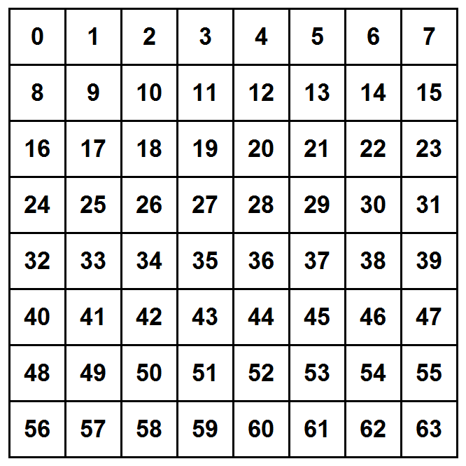
With this scheme, our neural network will have only 64 output neurons, which is not too bad. If you choose to work with this scheme, you will have to convert each defect point in our dataset to the corresponding region number in the training phase. It shouldn't be hard to find a simple formula for doing it. But again, feel free to explore other schemes (you may be forced to do so in case that your training dataset is insufficient for hitting precise locations of defects, so you might need to resort to coarser subdivisions)

# If you stick to the full 48x48 features scheme, then you will have 2304 classes
# Here is a simple way you can map pairs (i,j) to integers
classes = [48*i+j for i in range(48) for j in range(48)]

# This is a very long list, so we print the first 100 elements only:
print(classes[0:100])

[0, 1, 2, 3, 4, 5, 6, 7, 8, 9, 10, 11, 12, 13, 14, 15, 16, 17, 18, 19, 20, 21, 22, 23, 24, 25, 26, 27, 28, 29, 30, 31, 32, 33, 34, 35, 36, 37, 38, 39, 40, 41, 42, 43, 44, 45, 46, 47, 48, 49, 50, 51, 52, 53, 54, 55, 56, 57, 58, 59, 60, 61, 62, 63, 64, 65, 66, 67, 68, 69, 70, 71, 72, 73, 74, 75, 76, 77, 78, 79, 80, 81, 82, 83, 84, 85, 86, 87, 88, 89, 90, 91, 92, 93, 94, 95, 96, 97, 98, 99]

Data Exploration¶

Lets explore our HDF5 files to help you get started with your deep learning project.

We first show how to parse an HDF5 in order to extract the image and other circuit data.

from __future__ import print_function # we want to enable Python 3
import h5py
import numpy as np

# This is how you open an HDF5 file
f = h5py.File('opens1.h5', 'r')

# We will collect 2000 images (from th 80,000 images in this file) in one long Python list
images = []

# We will collect the first 2000 boxes
boxes = []

# And finally we will also collect the first 2000 defect centers
centers = []

# Our HDF5 file has a special key for the number of images which we're not going to use here
# but you will need it for the full project
# num_images = f.get('num_images').value

for i in range(2000):
    box_key = 'open_' + str(i)
    img_key = 'img_' + str(i)
    center_key = 'center_' + str(i)
    
    # This is the shape of the open defect
    box = np.array(f.get(box_key))
    boxes.append(box)
    
    # This is image i
    img = np.array(f.get(img_key))
    images.append(img)
    
    # This is the defect center data
    c = np.array(f.get(center_key))
    centers.append(c)

# Do not forget to close the HDF5 file!
f.close()

import matplotlib.pyplot as plt
from matplotlib import rcParams
%matplotlib inline

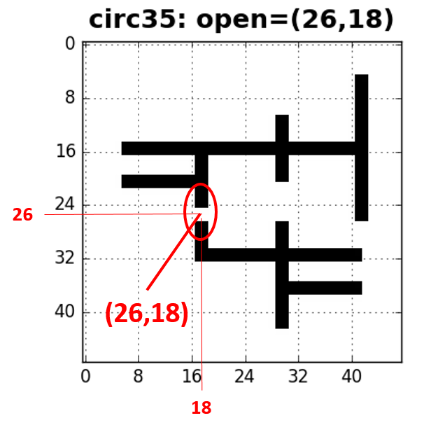
def draw_circ(i):
    print("Image id:", i)
    #print("Features:", hands[i])
    #c = box[i]
    img = images[i]
    x, y = centers[i]
    box = boxes[i]
    print("Box: %s" % (box,))
    print("Center: (%d,%d)" % (x,y))
    plt.title("circ%d: open=(%d,%d)" % (i,x,y), fontsize=18, fontweight='bold', y=1.02)
    ticks=[0,8,16,24,32,40, 48]
    plt.xticks(ticks, fontsize=12)
    plt.yticks(ticks, fontsize=12)
    plt.imshow(img, cmap='gray', interpolation='none')
    plt.plot(y, x, 'or')
    plt.grid()

Let's draw a few samples of circuits.

draw_circ(35)

Image id: 35
Box: [25 27 17 19]
Center: (26,18)

draw_circ(476)

Image id: 476
Box: [20 22 27 29]
Center: (21,28)

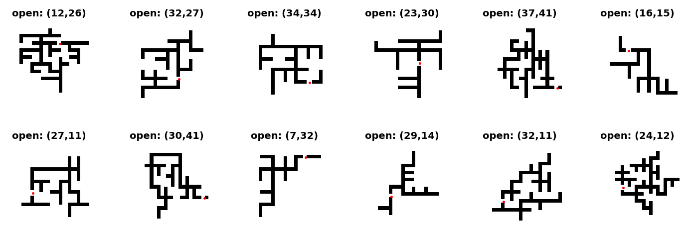
In some cases we need to view a larger group of samples at the same time. For example if we have a large group of false predictions, it is useful to look at a dozen or two of them in order to get a feeling about the kind of failure. The following function we draw a grid of mxn of circuits, m rows, n columns:

rcParams['figure.figsize'] = 9,9
def draw_group(imgs, cntrs, rows=4, cols=4):
    for i in range(0, rows*cols):
        ax = plt.subplot(rows, cols, i+1)
        img = imgs[i]
        x, y = cntrs[i]
        plt.title("circ%d: open=(%d,%d)" % (i,x,y), fontsize=8, fontweight='bold', y=1.02)
        ticks=[0,8,16,24,32,40, 48]
        plt.xticks(ticks, fontsize=7)
        plt.yticks(ticks, fontsize=7)
        plt.imshow(img, cmap='gray', interpolation='none')
        # adding a red marker for highlighting the open
        plt.plot(y, x, '.r', linewidth=0)
        plt.subplots_adjust(wspace=0.5, hspace=0.1)

draw_group(images[100:116], centers[100:116])

Class distribution (or class imbalance)¶

It is also highly recommended that you calculate the class distribution of your data. Try to count how many samples belong to each class. Like how many samples have an open defect at the point (32,15) (or in the region 17, if you go for the regions scheme). This is important to do in order to tune your expectations for model accuracy. The more the imbalance, the more chances that your model will be less accurate and biased. Therefore, you may need to carefully pick your training dataset from the above 400,000 samples. This task is of course part of this project ...

Your Mission¶

After building your training and validation sets (from the above 400,000 samples), deciding on a features scheme, your mission is to build a convolutional neural network for detecting the opens.

Make sure you don't use too many paramaters. Try to stay below half million.
Make sure you don't use too many layers. Try not to go beyond 12.
Make sure your model is trainable in a reasonable time. An upper bound of 10 to 20 hours is reasonable. Anythong beyond two days is unreasonable. This is assuming you are using a decent GPU card. Otherwise don't try it on your CPU (it can take forever).
Analyze the cases in which your model makes a false prediction