
This database is used as a cannonical example for several topics in data science and machine learning. The Pima indian diabetes dataset is originally from the National Institute of Diabetes and Digestive and Kidney Diseases. The objective is to predict if a patient has diabetes based on diagnostic measurements of eight simple features. We will also use this dataset for learning the basics of the Pandas library (which is essential for data science and machine learning).
Let's first start with listing the required Python modules for this project. We use the Keras deep learning library which makes things simple and practical. In a subsequent study unit we will also show how this can be done with Tensorflow.
Also note that we are using a designated module kerutils which contains some useful Keras and Numpy utilities for all our course units. It can be downloaded from: https://github.com/samyzaf/kerutils
from keras.models import Sequential, load_model
from keras.layers import Dense, Dropout, Activation, Flatten
from keras.layers.advanced_activations import PReLU, SReLU, ELU, LeakyReLU, ThresholdedReLU, ParametricSoftplus
from keras.layers.noise import GaussianNoise
from keras.utils.visualize_util import plot
import matplotlib.pyplot as plt
import matplotlib.cm
import pandas as pd
from pandas.tools.plotting import scatter_matrix
from kerutils import *

from matplotlib import rcParams
rcParams['axes.grid'] = True
rcParams['figure.figsize'] = 10,7
%matplotlib inline

# fixed random seed for reproducibility
np.random.seed(0)
from kerutils import *
# These are css/html styles for good looking ipython notebooks
from IPython.core.display import HTML
css = open('style-notebook.css').read()
HTML('<style>{}</style>'.format(css))
features = ['preg', 'plas', 'pres', 'skin', 'test', 'mass', 'pedi', 'age', 'class']
data = pd.read_csv('pima.csv', names=features)
# Lets view the first 10 rows of the data set
# See below what these names mean

data.head(10)
Medical Features short names
- preg = Number of times pregnant
- plas = Plasma glucose concentration a 2 hours in an oral glucose tolerance test
- pres = Diastolic blood pressure (mm Hg)
- skin = Triceps skin fold thickness (mm)
- test = 2-Hour serum insulin (mu U/ml)
- mass = Body mass index (weight in kg/(height in m)^2)
- pedi = Diabetes pedigree function
- age = Age (years)
- class = Class variable (1:tested positive for diabetes, 0: tested negative for diabetes)
More information: https://archive.ics.uci.edu/ml/datasets/Pima+Indians+Diabetes
# How many rows do we have?

data.index
# Try2: How many rows do we have?

len(data.index)
# How many columns do we have?

len(data.columns)
# How many records do we have in our data set?

data.size    # 9 * 768
# You can get everything in one line !

data.shape
# View the last 10 records of our data set

data.tail(10)
# The plot() method plots all features
# This is TMI (too much information)

data.plot()

# Better try one at a time
# Here is the plasma concentration level per record distribution
# (less is more!)

data.plot(y='plas')

# The graph above does not look very useful.
# Let's sort the plas values
plt.plot(sorted(data.plas.as_matrix()))

# This is the age distribution (sorted!)

plt.plot(sorted(data.age.as_matrix()))

# Age range

print("Min age = %d, Max age = %d" % (data.age.min(), data.age.max()))
# Age average

data.age.mean()
# Age median

data.age.median()
top = plt.subplot2grid((4,4), (0, 0), rowspan=2, colspan=4)
top.scatter(data['plas'], data['age'])
plt.title('Age against Plasma')
bottom = plt.subplot2grid((4,4), (2,0), rowspan=2, colspan=4)
bottom.bar(data['preg'], data['plas'])
plt.title('Plasma against Pregnancies')
plt.tight_layout()

Distribution by class=0 and class=1 (negative/positive diabetes test)
# Items with class == 0 (negative diabetes check)

data0 = data[data['class'] == 0]
len(data0.index)
# Items with class == 1 (persons with a positive diabtetes check)

data1 = data[data['class'] == 1]
len(data1.index)
# The Pandas groupby method computes the distribution of one feature
# with respect to the others
# We see 8 histograms distrubuted against a negative diabetes chck
# and other 8 histograms with distribution against a positive diabetes check

data.groupby('class').hist(figsize=(8,8), xlabelsize=7, ylabelsize=7)


sm = scatter_matrix(data, alpha=0.2, figsize=(7.5, 7.5), diagonal='kde')

[plt.setp(item.yaxis.get_majorticklabels(), 'size', 6) for item in sm.ravel()]
[plt.setp(item.xaxis.get_majorticklabels(), 'size', 6) for item in sm.ravel()]
plt.tight_layout(h_pad=0.15, w_pad=0.15)

Deep Learning with Keras
All the above Pandas coding and statistical charts are nice and helpful but in most practical situations are useless for coming up with an algorithm for predicting if a person is likely to have diabetes based on his 8 medical records.
In recent years, deep neural networks has been suggested as an effective technique for solving such problem, and so far has shown to be successful in many areas. We will try to build a simple neural network for predicting if a person has diabetes (0 or 1), based of the 8 features in his record. This is the full data except the class column! We want to be able to predict the class (positive or negative diabetes check) from the 8 features (as input)
#  Let's first extract the first 8 features from our data (from the 9 we have)
#  We want to be able to predict the class (positive or negative diabetes check)

X = data.ix[:,0:8]
# let's look at the first 10 records sample

X.head(10)
#This is the output class column!
Y = data.ix[:,8]
Y.head(10)
Keras Model Defintion

A sequential neural-network in Keras consists of a sequence of layers, starting from the inputs layer up to the output layer (also known as Feedforward Neural Network). The number and breadth of intermediate layers ("deep layers" or "hidden layers") depends on accuracy and performance requirements that we impose. We can start with a single hidden layer and add more neurons to it or add more hidden layers in progressive stages until we meet our accuracy requirements.
The second factor we need to attend is the connectivity type of our network: which neurons from a given layer are connected to which neurons at the next layer? The most straightforward type is full connectivity, which means that every neuron at a given layer is connected to every neuron at the next layer. This type of connectivity is reffered to by the Dense method of Keras layers module.
The third factor is what kind of activation function are we going to use? Each non-input neuron receives many inputs from neurons at the layer below it. How do we determine its output? The function that determines the value that a neuron fires in response to its inputs vector is called the activation function of the model.

Each connection must be assigned an initial weight, which is going to be tuned during the training phase. The usual arrangement is to assign small random weights when the model is defined. It usually has a negligible impact on the training speed.
The most common activation function used is the rectified linear unit (ReLU) function which is simply $$ \textbf{relu}(\vec{x}) = \max(\vec{w} \cdot \vec{x} + b, 0) $$ where $\vec{x}$ is the inputs vector, $\vec{w}$ is the weights vector, and $b$ is the bias value. In many experiments it has been determined that it is fast and leads to more accurate model.
For the output layer, the common practice is to use the sigmoid activation function as its output is always between 0 and 1 (which is useful for classifying). The sigmoid activation function is defined by: $$ \sigma(\vec{x}) = \frac{1}{1 + e^{-(\Sigma\vec{w} \cdot \vec{x} + b)}} \\ \hbox{ } $$ where $\vec{x}$ is the inputs vector, $\vec{w}$ is the weights vector, and $b$ is the bias value.
More information on activation functions is found here: http://stats.stackexchange.com/questions/115258/comprehensive-list-of-activation-functions-in-neural-networks-with-pros-cons
# Our first Keras Model
model1 = Sequential()
model1.add(Dense(16, input_shape=(8,), init='uniform', activation='relu'))
model1.add(Dense(1, init='uniform', activation='sigmoid'))
plot(model1, to_file='model1.png', show_shapes=True)


Compiling the model
After defining our model, we need to compile it to an efficient object code. If you own an advanced graphics card (GPU) like NVIDIA Tesla or Titan, then with proper configuration you will be able to run these nn models in a much faster and efficient manner than on a traditional Intel/AMD CPU.
Keras has two backends: Theano and Tensorflow (Google). Just recently, Tensorflow has been released to Microsoft Windows, but requires Python 3.5. Theano and Tensorflow are two important backend deep learning numerical engines that shall be covered in more detail later on ...
The Keras compile method accepts two important parameters: loss and optimizer.
A loss function role is to measure the distance from an actual output to the correct output (the error). It is the main source of feedback in the training process. Each time we run our model on a given input, the loss function measures the error of the output from the target objective. The main purpose of the training phase is to minimize the loss values. The standard choice is the logarithmic loss function which in Keras is reffered to as binary_crossentropy. The formula is: $$ \textbf{cross_entropy} (\vec{t}, \vec{o}) = - ( \vec{t} \cdot \log(\vec{o}) + (1 - \vec{t}) \cdot \log(1 - \vec{o})) $$ where $\vec{t}$ is the target vector and $\vec{o}$ is the model output vector.
The optimizer argument is a function which Keras is using for optimizing the model edge weights during the training process. Each time Keras finds a gap between the model output and the correct output, it tries to tune the weights of the model connections so as to minimize this gap as much as possible. This is a very delicate and highly intricate process that deserves a math course by itself. For our purposes it's enough to be familiar with its simplest form which in traditional math is called Stochastic Gradient Descent . Keras is using a specific variation which it calls adam. If needed, more information on this optimizer can be picked from here: https://arxiv.org/abs/1412.6980
The last parameter for the compile function is the metrics argument. It designates a method to judge the overall performance of our model by looking at large lists of outputs and targets. This is enough for the moment, it will be covered in more depth later on. Keras referrence: https://keras.io/metrics
model1.compile(loss='binary_crossentropy', optimizer='adam', metrics=['accuracy'])
Training our Model
After defining and compiling our model, it's time for training!
We will feed our model with many samples as inputs and their correct outputs.
Hopefully, after learning many real examples, our model will be capable of solving new cases.
- The training phase consists of several cycles (called epochs in Keras jargon), in which our training set is fed to it repeatedly. The number of epochs is up to you, and we may experiment with several options.
- In the training phase, our model will tune the weights of its edges. Keras provides an option to decide at which points the weights update is done through the batch_size argument. The weights update will occur after every batch_size training instances. Note that each epoch consists of the training of all test cases. We will try 200 epochs and a batch_size of 16.
- Our pima data set consists of 768 cases. We will use 668 of them for training and the remaining 100 cases for validation (testing).
X_train = X[0:668].as_matrix()
Y_train = Y[0:668].as_matrix()
X_test = X[668:].as_matrix()
Y_test = Y[668:].as_matrix()
FitMonitor
The FitMonitor callback is defined in the kerutils module and its purpose is to monitor the progress of the training process, report progress and some intermediate statistics, and save the best model in which the training accuracy and validations accuracy are maximal and are close enough (see 'filename' the 'thresh' parameters below).
fmon = FitMonitor()
And now the actual training is performed by the Keras Model fit method
h = model1.fit(
    X_train, Y_train,
    nb_epoch=100,
    batch_size=10,
    verbose=0,
    validation_data=(X_test, Y_test),
    callbacks=[fmon],
)
Saving the model to a file. It can be loaded later with the load_model method. Note that Keras uses the HDF5 file format to save the model.
model1.save("model_1.h5")
show_scores(model1, h, X_train, Y_train, X_test, Y_test)


# At any stage we can evaluate the accuracy and loss of our training set

loss, accuracy = model1.evaluate(X_train, Y_train, verbose=0)
print("Training: accuracy=%f, loss=%f" % (accuracy, loss))
# It is more interesting to evaluate our validation data
# and see if its scores resembles those of our training data

loss, accuracy = model1.evaluate(X_test, Y_test, verbose=0)
print("Validation: accuracy=%f, loss=%f" % (accuracy, loss))
The validation scores came out quite close to the training scores (this gap is usually an indication of an overfitting phenomenon which we will discuss more later on). In order to appreciate this result, we should ask ourselves what is the probability for it to happen? Just by looking at the data there doesn't seem to be any correlation between the validation set to the training set. The model was built by looking at the trainig data alone, and has not seen any of the test data at all. Theoretically, it well may happen that diabetes is a chaotic illness, and that there is no relation between the test data and the trainig data !?
Suppose we have $n$ records in our validation data X_test: ${x_1, x_2, x_3, \cdots, x_n}$. The probabilty for guessing the diabetes check for each record is $0.5$, and therefore the probability to guess more than 75% of the results is given by the formula $$ \textbf{probability} = \sum_{i=k}^{n} \binom{n}{i} \cdot p^{i} \cdot (1-p)^{n-i} $$ where $p = 0.5$ and $k = \textbf{int}(0.75 n)$. In our case, $n = 168$, $k = 117$, and $p = 0.5$.
A simple calculation yields: $$ \textbf{probabilty} = 3.0047541e-11 = 0.000000000030047541 $$
This is a convincing indication that the Pima Indian Diabetes database is indeed governed by some hidden laws which were partially captured by our neural-network (model1) but are not visible to the naked eye, not even for an experienced physician eye (I would even add and say that it would be foolish to trust a human to master the wisdom behind this data).
The amazing fact is that it took Keras 5 seconds to build the model1 neural-network, and it well maybe more trustable than some human trying to capture the database structure by a manual study of it.
Code for computing this probability can be obtained from
http://www.samyzaf.com/cgi-bin/view_file.py?file=ML/lib/prob.py
Trying model2 ...
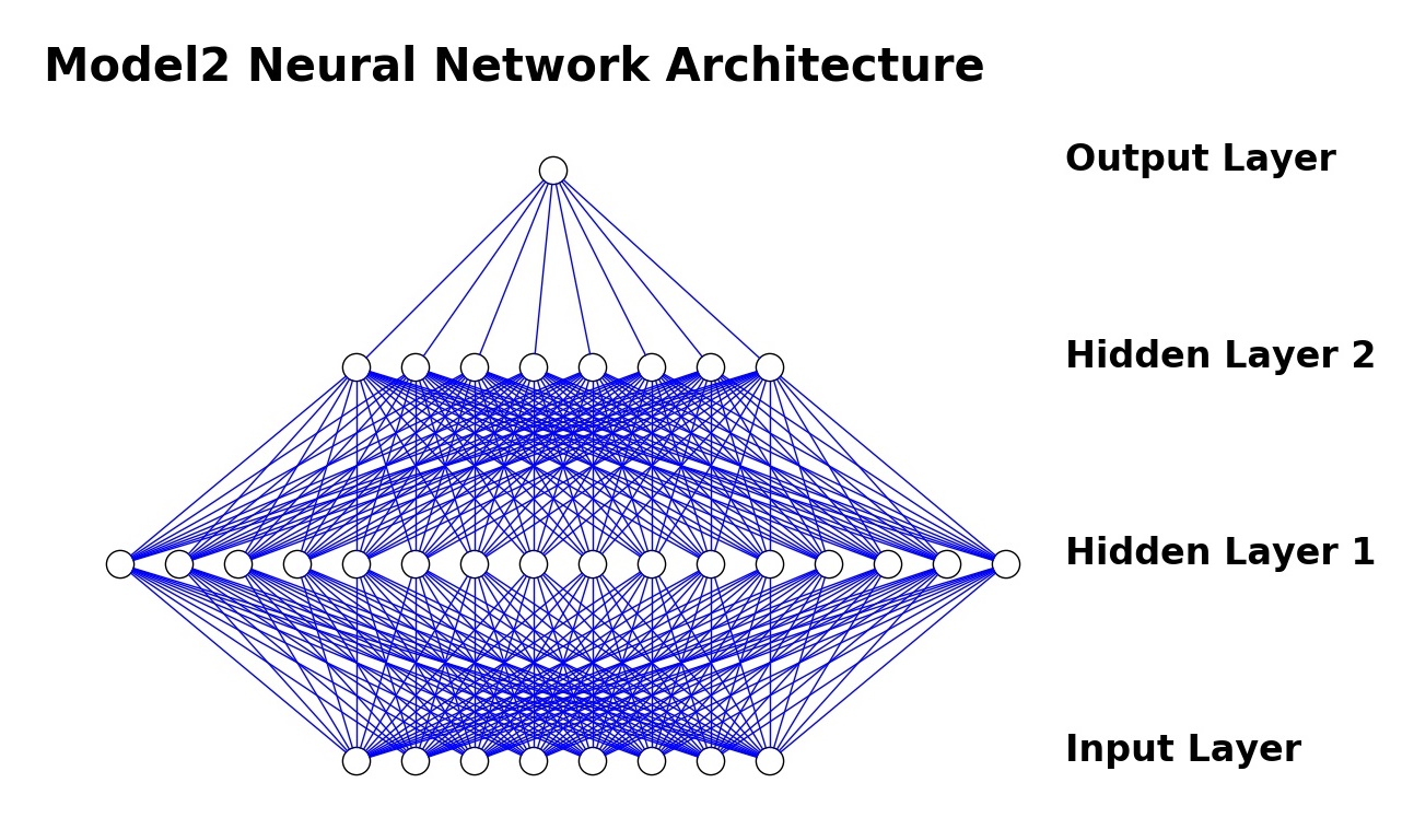
As model1 has shown an encouraging start. We will try now to add an additional deep layer with 8 neurons (just for curiosity testing) and build a new model2, which hopefully will be more successful than model1.
We will also increase the number of epochs (nb_epoch) to 160 and reduce batch_size to 8. We will try to capture the best model (in training process) whose training accuracy is not below 0.8 (minacc) and its distance to the validation accuracy (thresh) is below 0.05. If a model of this sort is found during the training process, it will be automatically saved in the file model_2_autosave.h5 (can happen several times).
# Our second Keras Model
model2 = Sequential()
model2.add(Dense(8, input_dim=8, init='uniform', activation='relu'))
model2.add(Dense(16, init='uniform', activation='relu'))
model2.add(Dense(1, init='uniform', activation='sigmoid'))

# compilation
model2.compile(loss='binary_crossentropy', optimizer='adam', metrics=['accuracy'])
# training
fmon = FitMonitor(thresh=0.05, minacc=0.8, filename="model_2_autosave.h5")
h = model2.fit(X_train, Y_train,
    nb_epoch=200,
    batch_size=16,
    validation_data=(X_test, Y_test),
    callbacks=[fmon],
    verbose=0,
)

model2.save("model_2.h5")
show_scores(model2, h, X_train, Y_train, X_test, Y_test)


Adding one more hidden layer improved accuracy slightly. The training and validation scores are even closer to each other which adds confidence to our model. However note that during the training process the FitMonitor was able to capture and save a model with a slightly better scores.
# We need to load the saved model which is better than the last one
model2 = load_model("model_2_autosave.h5")
# accuracy and loss of our training set

loss, accuracy = model2.evaluate(X_train, Y_train, verbose=0)
print("Train: accuracy=%f, loss=%f" % (accuracy, loss))
# accuracy and loss of validation set

loss, accuracy = model2.evaluate(X_test, Y_test, verbose=0)
print("Test: accuracy=%f, loss=%f" % (accuracy, loss))
Trying model 3
Model 2 has been a slight imporvement. Let us experiment with lots of neurons, and a different kind of activation function (leaky relu), just to get the hang of it. Note that Keras advanced activation functions are considered as layers (not functions), so they are specified in a separate line.
# Our third Keras Model
model3 = Sequential()
model3.add(Dense(8, input_dim=8, init='uniform'))
model3.add(LeakyReLU(0.2))
model3.add(Dense(64, init='uniform'))
model3.add(LeakyReLU(0.2))
model3.add(Dense(128, init='uniform'))
model3.add(LeakyReLU(0.2))
model3.add(Dense(64, init='uniform'))
model3.add(LeakyReLU(0.2))
model3.add(Dense(1, init='uniform', activation='sigmoid'))
model3.compile(loss='binary_crossentropy', optimizer='adam', metrics=['accuracy'])
fmon = FitMonitor(thresh=0.05, minacc=0.8, filename="model_3_autosave.h5")
h = model3.fit(
    X_train, Y_train,
    nb_epoch=300,
    batch_size=12,
    validation_data=(X_test, Y_test),
    callbacks=[fmon],
    verbose=0,
)

# model3.save("model_3.h5")
show_scores(model3, h, X_train, Y_train, X_test, Y_test)


# accuracy and loss of our training set

loss, accuracy = model3.evaluate(X_train, Y_train, verbose=0)
print("Train: accuracy=%f, loss=%f" % (accuracy, loss))
# accuracy and loss of testing set

loss, accuracy = model3.evaluate(X_test, Y_test, verbose=0)
print("Validation: accuracy=%f, loss=%f" % (accuracy, loss))
The training accuracy came out better (85.48% !) but the validation accuracy is a bit far behind, which means we are in an overfitting scenario. Our model is memorizing the training samples and is no good for other samples.
Most likely we will not be able to do better than this without more training data. Luckily, real medical databases usually contain larger sets of data that suffice for building efficient neural-networks. This is one of main lessons one learns each time: a neural network needs a lot of training samples. This is why it is important for institutions to collect as much data as possible.
Model 4
Sometimes, switching to a different activation function may help. Here is model 3 with the S-shaped linear rectifier (SReLU).
# Our 4th Keras Model
model4 = Sequential()
model4.add(Dense(8, input_dim=8, init='uniform'))
model4.add(SReLU())
model4.add(Dense(64, init='uniform'))
model4.add(SReLU())
model4.add(Dense(128, init='uniform'))
model4.add(SReLU())
model4.add(Dense(64, init='uniform'))
model4.add(SReLU())
model4.add(Dense(1, init='uniform', activation='sigmoid'))

model4.compile(loss='binary_crossentropy', optimizer='adam', metrics=['accuracy'])

fmon = FitMonitor(thresh=0.05, minacc=0.8, filename="model_4_autosave.h5")
h = model4.fit(
    X_train, Y_train,
    nb_epoch=300,
    batch_size=12,
    validation_data=(X_test, Y_test),
    callbacks=[fmon],
    verbose=0,
)

model4.save("model_4.h5")
show_scores(model4, h, X_train, Y_train, X_test, Y_test)


# accuracy and loss of our training set

loss, accuracy = model4.evaluate(X_train, Y_train, verbose=0)
print("Train: accuracy=%f, loss=%f" % (accuracy, loss))
# accuracy and loss of testing set

loss, accuracy = model4.evaluate(X_test, Y_test, verbose=0)
print("Validation: accuracy=%f, loss=%f" % (accuracy, loss))
The model accuracy graph looks better but the gap is still high. However the FitMonitor was able to capture a better model with a smaller gap.
model4 = load_model("model_4_autosave.h5")
# accuracy and loss of our training set

loss, accuracy = model4.evaluate(X_train, Y_train, verbose=0)
print("Train: accuracy=%f, loss=%f" % (accuracy, loss))
loss, accuracy = model4.evaluate(X_test, Y_test, verbose=0)
print("Test: accuracy=%f, loss=%f" % (accuracy, loss))
Model 5
Using the keras.callbacks.Callback mechanism it is possible to reverse engineer Keras for finding a network architecture with higher success rates. But it does require some programming and a long thorough search. There's always a risk of running into the pit of overfitting, in which the model is too large and can actually memorize the training set in it weights structure. We will conclude this study unit with a model that combines three different activation functions. They were randomly chosen but nevertheless seem to improve accuracy scores. We even get a higher validation score than training (which is sometimes called "underfitting", but is more desirable than overfitting).
model5 = Sequential()
model5.add(Dense(8, input_dim=8, init='uniform', activation='relu'))
model5.add(Dense(64, init='uniform'))
model4.add(SReLU())
model5.add(Dense(64, init='uniform'))
model5.add(LeakyReLU(0.05))
model5.add(Dense(64, init='uniform', activation='sigmoid'))
model5.add(Dense(1, init='uniform', activation='sigmoid'))

model5.compile(loss='binary_crossentropy', optimizer='adam', metrics=['accuracy'])

fmon = FitMonitor(thresh=0.05, minacc=0.8, filename="model_5_autosave.h5")
h = model5.fit(
    X_train, Y_train,
    nb_epoch=1024,
    batch_size=12,
    validation_data=(X_test, Y_test),
    callbacks=[fmon],
    verbose=0,
)

model5.save("model_5.h5")
show_scores(model5, h, X_train, Y_train, X_test, Y_test)


# accuracy and loss of our training set

loss, accuracy = model5.evaluate(X_train, Y_train, verbose=0)
print("Train: accuracy=%f, loss=%f" % (accuracy, loss))
# accuracy and loss of testing set

loss, accuracy = model5.evaluate(X_test, Y_test, verbose=0)
print("Validation: accuracy=%f, loss=%f" % (accuracy, loss))
Summary
So with a 265 neurons network we were able to define a neural network with about 81% accuracy scores. The question is can we do better? and are there systematic methods for improving neural network models? Currently this seems to be a wild area for creativity and imagination, and there are some web sites that conduct public competitions of this type. See for example: https://www.kaggle.com/competitions
Our course projects will follow these type of challenges, from which we believe the students can learn and get a lot of practice. It will also make the grading task much simpler :-) ...
Course Project 1
Find a minimal neural network for the Pima Indians database, which adhers to the following requirements:
- Produces at least 85% accuracy on the training and testing data sets
- Number of deep layers does not exceed 5
- Number of nuerons at each layer does not exceed 256
- Number of training epochs does not exceed 5000
- Number of parameters (weights) does not exceed 200K.
The solution with the smallest number of parameters will receive the highest grade, and the remaining solutions will receive smaller grades relative to their ranking compared to the best solution.
Course Project 2
Construct a minimal neural-network for predicting breast cancer reocurrence events. Accuracy should be at least 85%. The database can be downloaded from the university of California Irvine at: https://archive.ics.uci.edu/ml/datasets/Breast+Cancer
Course Project 3
Download the song_year database from: http://www.samyzaf.com/ML/song_year/song_year.zip. This database contains more than half million song records (515345) that were composed from 1922 to 2011. Each record consists of 91 features related to its audio attributes (including the year of its composition). Your task is to designed a neural-network that can predict the year from the other 90 musical attributes. Existence of such small network will be an indication that musical composition is strongly related to the time it is composed. Is this the case?